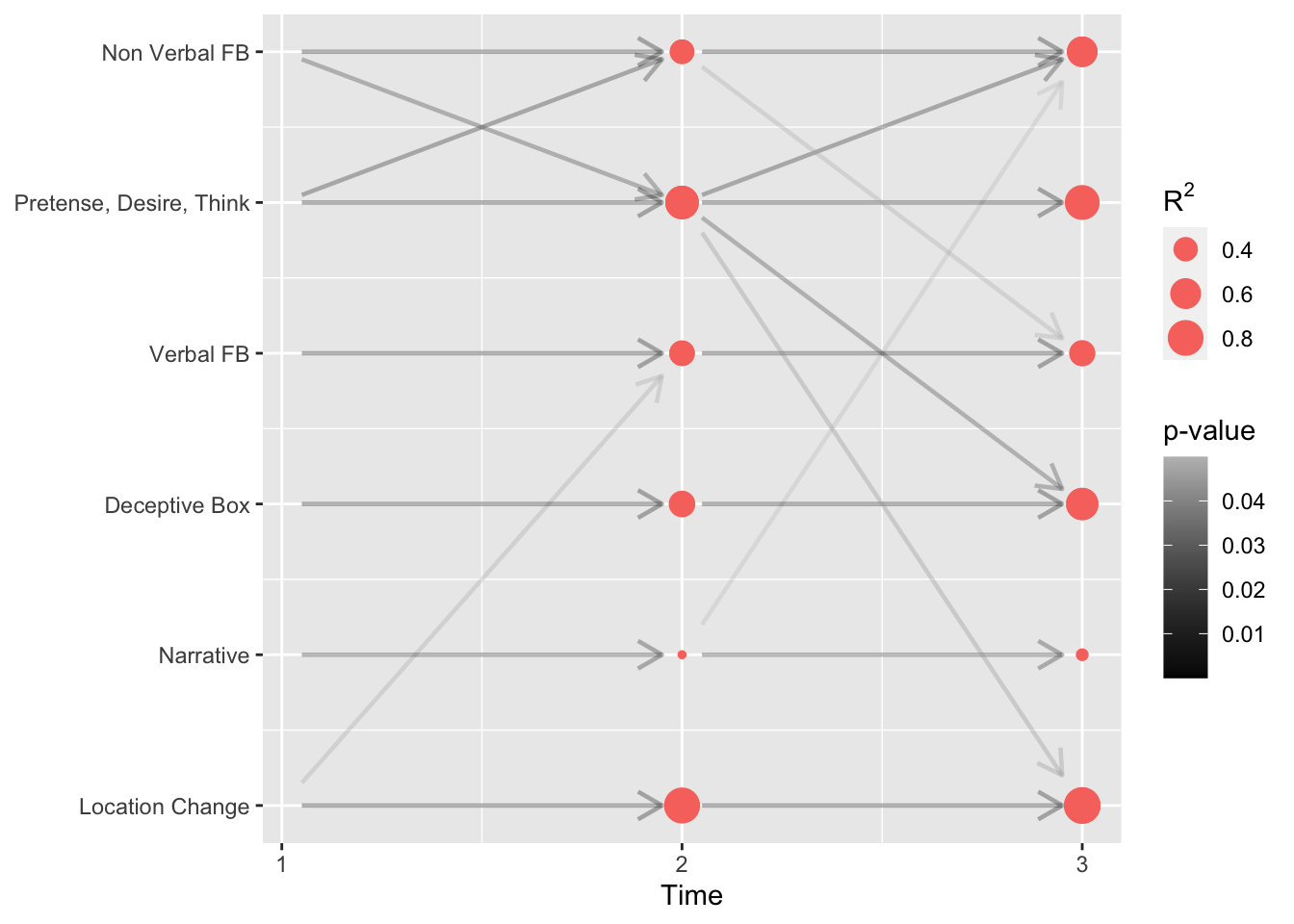
Causal Diagram
In this post, I would like to introduce a customized ggplot2 graphic that I did for my master dissertation. Basically, the plot will display how each latent ability found for Theory of Mind is affected by all the other abilities at previous times (we have information for three times). The process to find the latent abilities is not the main interest of the post, but it could be the topic for the next post. So let’s get back to the point.
Data
To obtain the data used for the path diagram, I employed a classical linear approach. Each latent ability at time 2 was regressed with all the abilities at time 1 including itself. Similarly, it was done for time 3 against time 2. Only the significant relations of each regression (p-value<0.05) were stored.
mydata <- read.table("data_causal.txt", header = TRUE, sep = "\t")
A small sample of the data is shown in the following table:
| x | xend | y | yend | pval | rsq | x2 | xend2 | y2 | yend2 |
|---|---|---|---|---|---|---|---|---|---|
| 1 | 2 | 6 | 6 | 0.000017 | 0.403304 | 1.05 | 1.95 | 6.00 | 6.00 |
| 1 | 2 | 5 | 6 | 0.004950 | 0.403304 | 1.05 | 1.95 | 5.05 | 5.95 |
| 2 | 3 | 5 | 1 | 0.041056 | 0.834008 | 2.05 | 2.95 | 4.80 | 1.20 |
| 2 | 3 | 1 | 1 | 0.000000 | 0.834008 | 2.05 | 2.95 | 1.00 | 1.00 |
- x is the departure time.
- xend is the arrival time.
- y is the ability (eg. 6 = Non Verbal False Belief, 1 = Location Change) considered as dependent variable in the regression at time x.
- yend is the ability considered as independent variable in the regression at time xend.
- pval is the p-value of the relation between y and yend.
- rsq is the coefficient of determination ($R^2$) of the regression.
The last four variables (x2, xend2, y2, yend2) were created based on the first ones to have a better location to be considered in the plot.
Plot
First, let’s define a function that will help us to choose a pretty color.
gg_color_hue <- function(n) {
  hues = seq(15, 375, length = n+1)
  hcl(h = hues, l = 65, c = 100)[1:n]
}
Finally, the code for the causal diagram is as follows:
library(ggplot2)

ggplot(mydata) +
  geom_segment(aes(x = x2, y = y2, xend = xend2, yend = yend2, col = pval), alpha = 0.3,
               arrow = arrow(length = unit(0.15,"inches")), size = 0.8) +
  scale_color_gradient(high = "gray", low = "black", name = "p-value") +
  geom_point(aes(x = xend, y = yend, size = rsq), col = gg_color_hue(4)[1]) +
  scale_x_continuous(breaks = 1:3) +
  scale_y_continuous(breaks = 1:6, labels = c("Location Change","Narrative","Deceptive Box",
                                              "Verbal FB","Pretense, Desire, Think",
                                              "Non Verbal FB")) +
  labs(x = "Time", y = NULL)  +
  guides(size = guide_legend(title = expression(R^2)))

Interpretation
The red shaded circles stands for the goodness of fit, which in linear models is the $R^2$, and it varies according to its value. Additionally, the darker the arrow is, the more significant becomes the precedent ability in explaining the respective latent ability at this time point.
It can be clearly seen that Pretense, Desire and Think can be explained at Time 2 by the same abilities and Non Verbal False Believe abilities had at Time 1. The same pattern is looked for Non Verbal False Belief at Time 2 which is summarised by its previous ability and the Pretense, Desire and Think ability at Time 1. However, these last causality is less accurate since its $R^2$ value is smaller. Even though there is an arrow from Location Change ability at Time 1 to Verbal False Belief ability at Time 2 indicating causality, it is not that much significant ($p-value \approx 0.05$) and also the $R^2$ is around 50%. The remaining abilities at Time 2 are as well explained by themselves at Time 1.
At Time 3, all the abilities are caused by their previous time point value. The remarkable pattern is shown by Pretense, Desire and Think at Time 2 explaining three dimensions at Time 3 apart form itself: Non Verbal False Belief, Dceptive Box and Location Change. These last with not a strong p-value but it still having a good precision ($R^2$ around 0.8). Moreover, Non Verbal False Belief ability seem to be explained also by the Narrative factor, but the significance is almost at the boundary and can be because the p-values, in general, have not been adjusted for multiple comparison.